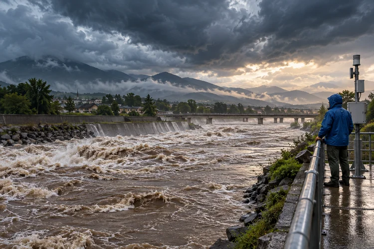
Imagine watching a peaceful river suddenly transform into a powerful, fast-moving stream after several hours of heavy rainfall.
Water levels rise, velocities change, and flood waves travel downstream, sometimes creating unexpected problems for nearby communities and infrastructure.
Predicting these changes isn’t as simple as measuring how much water enters a channel.
Water movement depends on several interconnected factors, including channel geometry, bed slope, surface roughness, rainfall intensity, and downstream conditions. These variables can change throughout a storm, making hydraulic predictions surprisingly complicated.
That’s where numerical modeling strategies for unsteady open channel flows become incredibly useful.
Instead of relying on simplified assumptions about constant water movement, numerical simulations calculate how flow depth, discharge, and velocity evolve across space and time.
Engineers use these models to investigate flooding, evaluate river restoration projects, design drainage infrastructure, and assess the performance of hydraulic structures.
However, building an accurate simulation requires more than choosing sophisticated software.
You need the right governing equations, computational methods, boundary conditions, and validation techniques.
In this guide, we’ll explore practical approaches for developing reliable, efficient, and realistic unsteady flow simulations without making the mathematics unnecessarily complicated.
1. Understanding Unsteady Open Channel Flow Dynamics
Before jumping into numerical algorithms, it’s important to understand what makes unsteady flow different from ordinary steady-state hydraulics.
In steady flow, hydraulic conditions at a particular location remain constant over time. Water depth and discharge may vary along the channel, but they don’t change at a fixed point.
Unsteady flow behaves differently.
Discharge, velocity, and water surface elevation change with time, often while also varying along the channel.
Why Unsteady Flow Matters
Consider a river receiving runoff from an intense upstream storm.
At first, downstream water levels may remain relatively low. As the flood wave travels through the river system, discharge increases, the water surface rises, and the channel begins storing additional water.
Eventually, the flood peak passes and water levels gradually decrease.
This entire process involves changing hydraulic conditions that cannot be fully represented by a single steady-state calculation.
Unsteady simulations are particularly important when analyzing rapid flood waves, dam releases, tidal backwater, stormwater surges, and operational changes at hydraulic structures.
The Role of Flow Regimes
The Froude number helps engineers identify different flow behaviors.
It compares flow velocity with the speed of gravity waves:
[
Fr=\frac{V}{\sqrt{gD}}
]
Here, (V) represents mean velocity, (g) is gravitational acceleration, and (D) is hydraulic depth.
Subcritical flow occurs when the Froude number is below one, while supercritical flow occurs when it exceeds one.
Near critical flow, small changes in channel geometry or discharge can cause major changes in hydraulic behavior.
Understanding these regimes helps engineers select numerical methods capable of handling wave propagation, hydraulic jumps, and rapidly changing conditions.
2. Choosing the Right Governing Equations
Every hydraulic simulation begins with mathematical equations describing how water moves.
For unsteady open channels, the most widely used framework is the Saint-Venant equations, which represent conservation of mass and momentum.
These equations provide the foundation for many modern river modeling applications.
The Saint-Venant Equations
The one-dimensional continuity equation can be written as:
[
\frac{\partial A}{\partial t}+\frac{\partial Q}{\partial x}=q_l
]
Here, (A) is the flow area, (Q) is discharge, (t) represents time, (x) is the longitudinal distance, and (q_l) represents lateral inflow per unit channel length.
In simple terms, the equation tracks how water enters, leaves, and accumulates within a channel segment.
For a prismatic channel under common one-dimensional assumptions, the momentum equation can be expressed as:
[
\frac{\partial Q}{\partial t}
+\frac{\partial}{\partial x}\left(\frac{Q^2}{A}\right)
+gA\frac{\partial h}{\partial x}
=gA(S_0-S_f)
]
Here, (h) is water depth, (S_0) represents bed slope, and (S_f) represents friction slope.
Additional geometry, momentum correction, and lateral inflow terms may be necessary for more general river systems.
Together, these equations describe acceleration, pressure forces, gravity, and frictional resistance.
Kinematic, Diffusion, and Dynamic Wave Models
Not every project requires the complete momentum equation.
A kinematic wave model simplifies the physics by assuming that gravitational driving forces are primarily balanced by friction.
This approach works well for some gradually varying flows in relatively steep channels where backwater and inertia are unimportant.
Diffusion wave models retain the effects of water surface gradients, allowing them to represent backwater-related spreading more realistically.
However, they neglect important acceleration terms.
Full dynamic wave models include local and convective acceleration, making them more appropriate for rapidly changing conditions, flow reversals, and complex hydraulic interactions.
The key is matching the equations to the actual problem.
Using the most complicated model isn’t automatically the smartest decision, especially when simpler equations can answer the engineering question accurately.
3. Selecting Effective Numerical Solution Methods
Even with the correct governing equations, obtaining a numerical solution presents another challenge.
Real rivers have irregular cross sections, varying slopes, complicated boundaries, and changing water depths.
Analytical solutions rarely exist for these conditions, so engineers divide the system into smaller computational elements and solve approximate equations.
Finite Difference Methods
Finite difference methods approximate derivatives using values at discrete points.
They are particularly useful for one-dimensional river routing, where the channel can be represented by a sequence of cross sections.
Implicit finite difference schemes, including the well-known Preissmann box method, are widely used in unsteady hydraulic calculations.
Their main advantage is numerical stability over comparatively large time steps.
However, large time steps can still introduce significant numerical damping or reduce the accuracy of rapidly changing flood waves.
This distinction matters: a simulation that runs without crashing isn’t necessarily producing trustworthy results.
Finite Volume Methods
Finite volume methods approach the problem differently.
Instead of focusing primarily on derivatives at individual points, they calculate how mass and momentum move across the boundaries of computational cells.
Because each cell accounts for incoming and outgoing fluxes, these methods are particularly attractive for conservation-based hydraulic modeling.
They are widely used in two-dimensional shallow water solvers and can handle rapidly varying conditions when suitable flux calculations are implemented.
Godunov-type schemes and approximate Riemann solvers, such as HLL and HLLC, are common examples.
These methods can capture sharp transitions more effectively than some traditional discretization approaches.
Explicit Versus Implicit Time Integration
Explicit methods calculate the next solution using information already available at the current time step.
They can be straightforward and computationally efficient per step, but their stable time-step size is often restricted.
Implicit methods solve equations involving unknown values at the next time level.
They generally require more computation per step but can sometimes operate with larger intervals.
Interestingly, a simplified inertial formulation proposed by Bates, Horritt, and Fewtrell in 2010 demonstrated how reduced shallow water equations could support efficient two-dimensional flood simulations.
The broader lesson is simple: computational efficiency often comes from choosing appropriate physics and numerical approximations, not just purchasing faster hardware.
4. Building Better Computational Grids and Time Steps
A numerical solver is only as useful as the spatial representation supporting it.
If your computational grid overlooks important hydraulic features, even an advanced algorithm may produce misleading results.
Choosing an Appropriate Mesh Resolution
One-dimensional models generally use river cross sections connected along the flow direction.
Two-dimensional models divide floodplains and channels into computational cells.
Smaller cells provide greater spatial detail but increase computational requirements.
For example, a floodplain represented by 40-meter square cells may require approximately four times as many cells if resolution is reduced to 20 meters in both horizontal directions.
The computational cost can increase further when the smaller cells require shorter time steps.
This is why uniform high-resolution meshing isn’t always the best approch.
Instead, focus detailed cells around bridges, levees, sharp bends, channel transitions, and densely developed floodplains.
Coarser cells may be suitable for wide, relatively uniform areas where flow gradients are smaller.
Why Terrain Data Matters
A detailed mesh cannot compensate for inaccurate topography.
Digital elevation models, surveyed river cross sections, and bathymetric measurements determine how the simulated water moves through the landscape.
LiDAR-derived terrain can capture detailed floodplain elevations, but it may not accurately represent submerged riverbeds.
Additional bathymetric surveys are often needed.
Breaklines also help align computational cell faces with levees, roads, embankments, and other features controlling water movement.
Managing the Courant Number
Time-step selection is another major consideration.
For a simple explicit shallow water solver, a common stability condition involves the Courant-Friedrichs-Lewy criterion:
[
C=\frac{(|u|+\sqrt{gh})\Delta t}{\Delta x}
]
Here, (\Delta t) represents the time step, (\Delta x) is cell size, and (u) is velocity along the relevant direction.
Suppose a model uses 20-meter cells, a water depth of 2 meters, and a velocity of 2 meters per second.
The corresponding characteristic wave speed is approximately 6.43 meters per second.
A one-dimensional CFL limit of one would suggest a maximum time step of approximately 3.1 seconds.
The precise limit depends on the solver, mesh geometry, and integration method, but this example demonstrates why smaller cells can require more frequent computations.
5. Defining Realistic Boundary and Initial Conditions
Even an excellent numerical scheme cannot overcome unrealistic input conditions.
Boundary conditions determine how water enters and leaves the modeled system, while initial conditions describe the hydraulic state before calculations begin.
Getting both right is essential.
Upstream and Downstream Boundaries
An upstream flow hydrograph commonly specifies how discharge changes throughout a simulation.
For example, a hypothetical storm event might increase river discharge from 100 to 250 cubic meters per second over several hours.
The model uses this time series to calculate how the flood wave propagates downstream.
Downstream boundaries may use recorded water levels, rating curves, normal-depth assumptions, or other hydraulic relationships.
Their suitability depends on channel conditions and the expected flow regime.
A downstream boundary placed too close to the study area can distort predicted water levels, especially when backwater effects are significant.
Initial Water Levels and Warm-Up Periods
Initial conditions deserve just as much attention.
Starting a model with an unrealistic dry channel or inconsistent water surface elevation can generate artificial disturbances.
These disturbances may be mistaken for actual flood-wave behavior.
A model warm-up period allows the hydraulic solution to adjust before the period of interest begins.
For complex river networks, this can substantially improve simulation consistency.
Representing Hydraulic Structures
Bridges, gates, culverts, and weirs can strongly influence unsteady flow patterns.
Their geometry and hydraulic characteristics should be represented using suitable structure formulations or carefully resolved computational geometry.
Ignoring these features may underestimate upstream water levels or misrepresent local velocities.
When multiple structures interact, their combined influence can become especially important during extreme events.
This is becuase local restrictions may affect both flood-wave timing and upstream storage.
6. Calibrating and Validating Hydraulic Simulations
Building a model is one thing. Demonstrating that it represents real-world hydraulic behavior is another.
Calibration and validation help establish whether simulation results are credible enough for engineering decisions.
Calibrating Hydraulic Parameters
Calibration involves adjusting uncertain model parameters so simulated results reasonably reproduce observations.
Manning’s roughness coefficient is one of the most influential parameters in open channel hydraulics.
It represents resistance associated with channel surfaces, vegetation, irregularities, and other flow-retarding features.
However, roughness should not become a convenient tool for hiding poor terrain data or incorrect boundary conditions.
If simulated water levels are consistently too high, the problem might involve excessive roughness, inaccurate channel geometry, or an inappropriate downstream boundary.
Changing Manning’s coefficient without investigating these possibilities can create misleading improvements.
Evaluating Model Performance
A useful calibration process compares simulated and observed water surface elevations, discharges, and flood-wave timing.
Engineers often examine peak-stage error, peak-flow error, travel-time differences, and overall hydrograph shape.
Statistical measures such as root mean square error, mean absolute error, and Nash-Sutcliffe efficiency can provide additional insight.
However, no single metric tells the entire story.
A model might reproduce peak water levels accurately while predicting the peak several hours too early.
For flood forecasting, that timing error could be highly significant.
Validation and Uncertainty Analysis
After calibration, test the model against independent events that were not used to adjust its parameters.
This helps determine whether the model performs consistently under different hydraulic conditions.
Sensitivity analysis adds another layer of reliability.
For example, changing roughness values, inflow estimates, or downstream conditions within plausible ranges reveals how much the predictions depend on uncertain assumptions.
A consistant modeling workflow should also evaluate uncertainty in terrain elevation and channel geometry.
Instead of reporting a single flood extent as an absolute prediction, engineers can compare multiple plausible scenarios.
This provides a more useful picture of potential hydraulic risk.
7. Improving Computational Efficiency Without Sacrificing Accuracy
High-resolution hydraulic simulations can become computationally expensive, particularly when thousands or millions of cells are involved.
Fortunately, improving performance doesn’t always require reducing model quality.
Combining 1D and 2D Modeling
Hybrid modeling is one practical solution.
One-dimensional calculations can represent long river reaches where flow is primarily aligned with the channel.
Two-dimensional calculations can then represent locations where lateral flow distribution is important, such as urban floodplains and complicated river junctions.
Imagine modeling a 15-kilometer river with a densely developed town near its midpoint.
Instead of applying a detailed two-dimensional grid across the entire watershed, engineers might use 1D routing upstream and downstream while applying 2D hydraulics around the town.
The transition between models must conserve flow and represent water exchange accurately.
When implemented carefully, this approach can provide useful spatial detail without unnecessary computational expense.
Adaptive Time Stepping and Solver Settings
Adaptive time stepping allows the solver to adjust computational intervals as hydraulic conditions change.
Relatively calm conditions may permit larger steps, while rapidly changing flood waves require smaller ones.
Some hydraulic software also provides control over convergence tolerances, iteration limits, and numerical solution options.
Adjusting these settings can improve computational efficiency, but changes should always be tested against solution accuracy.
Solver-specific guidance matters, especially becuase different algorithms have different stability requirements.
Verification Before Large Simulations
Before running a complete design event, perform smaller verification tests.
Check whether the model conserves mass, maintains reasonable water depths, and produces stable hydrographs.
For example, if a hypothetical simulation receives one million cubic meters of water, releases 900,000 cubic meters, and stores another 100,000 cubic meters, its volume balance closes.
Real models may also include rainfall, infiltration, and other source or sink terms.
Unexpected volume discrepancies can indicate numerical problems, incorrect boundary settings, or missing flow pathways.
Running a mesh sensitivity study is equally useful.
If further refinement causes only minor changes in relevant results, additional computational detail may offer limited practical benefits.
Ultimately, the goal isn’t to create the biggest hydraulic model possible.
It’s to create the smallest reliable model capable of answering the engineering question.
Numerical modeling of unsteady open channel flows provides a powerful way to understand how rivers, canals, and drainage systems respond to changing hydraulic conditions.
Reliable predictions depend on choosing suitable governing equations, selecting stable numerical methods, developing accurate computational grids, and applying realistic boundary conditions.
Calibration, independent validation, and uncertainty analysis are equally important for producing results engineers can confidently interpret.
Perhaps the most valuable strategy is finding the right balance between physical realism and computational efficiency.
A well-designed simulation doesn’t need unnecessary complexity to deliver meaningful insights.
Ready to improve your next hydraulic modeling project? Start by reviewing your model assumptions, checking terrain quality, and testing numerical sensitivity before increasing resolution.
These practical improvements can make a significant difference in the reliability of flood predictions and hydraulic design decisions.