Rivers are surprisingly complicated. What looks like a simple stream of moving water is actually a constantly changing system influenced by gravity, terrain, turbulence, sediment, and countless environmental factors.
Now imagine trying to predict exactly how that water will behave during extreme rainfall, around a sharp river bend, or beneath a newly constructed bridge. Suddenly, things become much more challenging.
That’s where advanced computational hydraulics for complex river flow models comes into play.
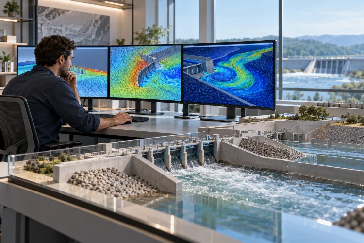
By combining mathematical equations, numerical simulations, and high-resolution geographic data, engineers can recreate river behavior inside a virtual environment.
Instead of relying entirely on physical experiments or simplified calculations, they can investigate different flow conditions before making expensive engineering decisions.
Modern hydraulic modeling technologies also make it possible to visualize flood patterns, estimate water velocities, examine erosion risks, and evaluate hydraulic infrastructure under different scenarios.
But creating an accurate river flow model isn’t simply about running sophisticated software. It requires a solid understanding of fluid mechanics, reliable input data, appropriate numerical methods, and careful validation.
Let’s explore how these technologies work, why they matter, and how engineers can use them to build more reliable river simulations.
1. Why Complex River Systems Need Advanced Hydraulic Modeling
A river rarely behaves like a perfectly straight channel with uniform water movement.
Natural waterways contain bends, changing depths, irregular banks, vegetation, bridges, sediment deposits, and floodplains. Each feature influences how water moves through the system.
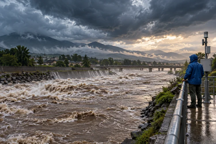
During normal flow conditions, these influences might seem relatively manageable. However, when river discharge increases rapidly, even minor geometric variations can create significant changes in water levels and velocity distributions.
For example, water approaching a narrow bridge opening may accelerate as it passes through the restricted area. Depending on the hydraulic conditions, the bridge can also produce upstream backwater effects, localized turbulence, and increased erosion potential.
Traditional hydraulic calculations can estimate many of these effects, but simplified approaches often struggle to represent complicated spatial interactions.
Moving Beyond Simplified River Calculations
Conventional one-dimensional hydraulic models generally describe flow primarily along the river’s longitudinal direction.
They remain useful for many engineering applications, particularly when flow movement follows a clearly defined channel.
However, complex river environments sometimes require more detailed information.
Imagine a flood spreading across an agricultural floodplain. Water may travel downstream, move sideways between fields, pass through road openings, and eventually reconnect with the main river.
A two-dimensional model can represent these horizontal flow pathways more explicitly than a conventional 1D approach.
For even greater detail, three-dimensional simulations can examine vertical velocity variations, secondary circulation, and localized turbulence.
The important takeaway? A more advanced model should be selected because the engineering problem requires it, not simply because the software offers it.
2. Understanding the Physics Behind Computational River Models
At the heart of computational river hydraulics are mathematical equations describing the movement of water.
These equations follow fundamental physical principles, including conservation of mass and conservation of momentum.
In simple terms, water cannot mysteriously disappear from a modeled system, and changes in its movement must be explained by forces acting on it.
Shallow Water Equations and Flow Dynamics
Many river simulations rely on the shallow water equations, which represent the movement of water using depth-averaged hydraulic variables.
These equations are especially useful when horizontal flow dimensions are much larger than water depth.
They allow engineers to estimate important parameters such as water-surface elevation, flow velocity, discharge distribution, and flood propagation.
For example, consider a river section experiencing a sudden increase in upstream discharge.
A depth-averaged model can simulate how the resulting flood wave travels downstream, interacts with channel geometry, and spreads into adjacent low-lying areas.
This approach offers a practical balance between computational efficiency and physical accuracy.
When Three-Dimensional CFD Becomes Necessary
Some hydraulic problems require a deeper look into the actual structure of flowing water.
This is where Computational Fluid Dynamics, or CFD, becomes particularly valuable.
Three-dimensional CFD models commonly solve the Navier–Stokes equations, often using turbulence-modeling techniques to make complex calculations computationally manageable.
These simulations can reveal vertical circulation, recirculation zones, and turbulent structures that depth-averaged models cannot fully resolve.
Consider a bridge pier positioned in a fast-flowing river.
Water accelerates around the structure, generating complicated vortices that can contribute to local scour. A carefully configured 3D model can help engineers investigate the associated flow patterns.
Common turbulence approaches include Reynolds-Averaged Navier–Stokes (RANS) models and Large Eddy Simulation (LES).
RANS generally offers a more economical way to estimate turbulent flow characteristics, while LES resolves larger turbulent structures at a considerably higher computational cost.
For most river-scale flood studies, 2D modeling remains a sensible starting point. Detailed 3D CFD is often reserved for locations where vertical flow structure matters.
3. Building Reliable River Models With High-Quality Input Data
Even the most sophisticated hydraulic solver cannot compensate for inaccurate environmental information.
A river model is only as reliable as the geometry, boundary conditions, and hydraulic parameters used to construct it.
That’s why data preparation is one of the most important parts of any numerical modeling project.
Terrain Elevation and River Bathymetry
Digital Elevation Models (DEMs) describe the surrounding land surface.
They help identify floodplains, embankments, drainage corridors, and other features that influence inundation.
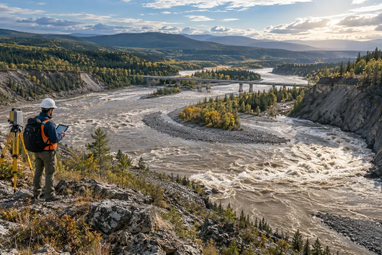
High-resolution LiDAR surveys can provide detailed terrain information, making them valuable for modern flood simulations.
However, ordinary topographic LiDAR generally cannot measure submerged riverbeds.
Engineers often combine terrestrial elevation data with bathymetric surveys obtained through sonar, acoustic instruments, or specialized green-wavelength bathymetric LiDAR.
A useful example comes from a 2026 U.S. Geological Survey data release covering the Santiam River Basin in Oregon.
The survey included approximately 125 kilometers of river reaches. Bathymetric LiDAR generally measured channel areas shallower than three meters, while sonar measurements helped fill gaps in deeper sections.
This example highlights an important principle: different measurement technologies frequently need to work together to describe an entire river system accurately.
Boundary Conditions and Hydraulic Parameters
Geometry alone doesn’t tell the model how water enters, moves through, or leaves the computational domain.
Engineers must also define appropriate hydraulic boundary conditions.
An upstream flow hydrograph might describe how discharge changes during a storm, while a downstream stage hydrograph specifies changing water levels.
Additional inputs may include tributary inflows, rainfall, hydraulic structures, and initial water levels.
Bed friction is another critical factor.
Manning’s roughness coefficient, commonly represented as n, describes resistance associated with channel and floodplain surfaces.
A smooth, relatively unobstructed channel generally behaves differently from a river covered with dense vegetation, irregular stones, or woody debris.
Choosing realistic roughness values is essential because they influence simulated water levels and velocity.
An incorrect boundry condition or roughness assumption can distort results across a large portion of the computational domain.
4. Improving Simulation Accuracy Through Mesh Design and Numerical Methods
One of the most interesting aspects of computational hydraulics is how a physical river gets converted into something a computer can calculate.
The process involves dividing the modeling area into smaller computational elements, collectively known as a mesh.
Each element represents a portion of the river or floodplain where hydraulic equations are solved.
Finding the Right Mesh Resolution
A finer mesh can represent localized hydraulic changes more effectively, but it also increases computational demands.
Imagine modeling a two-square-kilometer floodplain using square computational cells.
With 20-meter cells, the domain contains approximately 5,000 cells.
Reducing the cell width to five meters increases that number to approximately 80,000.
Illustrative calculation assuming a uniform square grid and identical domain area.
That’s sixteen times as many cells, even before considering additional numerical costs.
Therefore, extremely fine meshes aren’t automatically the best choice.
A smarter approach involves applying smaller elements near important hydraulic features while retaining larger cells in relatively uniform areas.
For example, engineers might refine the mesh around bridge openings, levees, sharp bends, and narrow floodplain connections.
According to the U.S. Army Corps of Engineers’ HEC-RAS documentation, computational meshes can use structured or unstructured cells, with underlying terrain information supporting the representation of important hydraulic characteristics.
This flexibility makes it possible to balance geometric detail and simulation efficiency.
Time Steps, Stability, and Numerical Accuracy
Spatial resolution is only one part of the equation.
Hydraulic models also calculate how flow conditions evolve over time.
The interval between successive calculations is called the computational time step.
If a model uses excessively large time steps, rapidly changing flow behavior may not be represented adequately. Certain numerical schemes may also become unstable.
For explicit shallow-water solvers, the Courant–Friedrichs–Lewy (CFL) condition provides an important stability consideration.
The allowable time step depends on cell dimensions, local velocity, wave speed, and the numerical method.
Implicit solvers may tolerate larger time steps, although larger intervals can still reduce temporal accuracy.
A practical strategy is to test several mesh resolutions and time-step settings, then compare the results.
When further refinement produces only small changes in the outputs that matter, engineers gain greater confidence in the numerical resoultion.
5. Calibration, Validation, and Uncertainty in Hydraulic Simulations
A model that produces beautiful water-depth maps isn’t necessarily accurate.
To determine whether a numerical simulation represents real hydraulic behavior, engineers must compare its predictions with observed measurements.
This process involves calibration and validation.
Matching Simulation Results With Field Measurements
Calibration involves adjusting uncertain model parameters within defensible physical ranges.
For example, engineers may refine bed roughness assumptions to improve agreement between simulated and measured water-surface elevations.
Other observations can include discharge records, flow velocities, flood extents, and water depths.
A real-world example comes from a U.S. Geological Survey investigation of the Ohio River near Jefferson County, Kentucky.
Researchers calibrated a two-dimensional hydrodynamic model using observations collected at approximately 35,000 cubic feet per second and verified it against higher-flow observations of approximately 390,000 cubic feet per second.
The study compared water-surface elevations at ten locations and velocity profiles across thirty cross sections.
This demonstrates how field observations can provide a measurable basis for evaluating numerical predictions.
Importantly, validation should use independent observations rather than relying entirely on the same dataset used during calbration.
Understanding Model Uncertainty
Every hydraulic simulation contains uncertainty.
Some uncertainties originate from incomplete terrain measurements, while others involve flow estimates, roughness parameters, numerical approximations, or future environmental conditions.
The U.S. Geological Survey has identified hydrologic inputs, terrain information, and hydraulic model characteristics as important sources of uncertainty in flood inundation mapping.
Engineers can investigate these influences through sensitivity analysis.
For example, a project team might run multiple scenarios using different plausible roughness values or upstream discharge estimates.
If a small input adjustment produces a large change in predicted flood depth, that area deserves additional investigation.
Quantitative evaluation can also help.
Root Mean Square Error (RMSE) can summarize differences between observed and simulated water levels, while spatial overlap metrics can evaluate predicted flood boundaries.
The goal isn’t to create a mathematically perfect river representation.
It’s to develop a model that is sufficiently reliable, transparent, and appropriate for its intended engineering decisions.
6. Real-World Applications of Advanced River Flow Simulations
Computational hydraulics becomes especially valuable when model outputs support practical decisions.
From flood management to ecological restoration, numerical simulations provide a way to investigate scenarios that would be expensive or dangerous to reproduce physically.
Flood Risk Assessment and Inundation Mapping
Flood modeling is one of the most common applications.
Engineers can simulate different storm scenarios, river discharge conditions, and infrastructure configurations to estimate where water may spread.
The resulting outputs can include flood depth, velocity, inundation extent, and arrival time.
These predictions help communities identify vulnerable roads, buildings, farmland, and critical infrastructure.
Consider a proposed flood protection embankment.
A hydraulic simluation can help determine whether the structure reduces inundation in the target area or unintentionally redirects water toward neighboring communities.
This information is valuable before construction begins.
Bridge Design, Erosion, and River Restoration
Hydraulic simulations also support bridge and river engineering projects.
For bridges, detailed modeling can help identify regions of accelerated flow and potentially damaging turbulence.
However, predicting actual scour depths generally requires additional sediment-transport analysis, empirical relationships, or specialized scour modeling.
In restoration projects, engineers may simulate alternative channel layouts, reconnect floodplains, or investigate habitat conditions under different discharges.
For example, varying water depth and velocity can influence the suitability of particular river areas for aquatic organisms.
Sediment transport models can extend these investigations by estimating erosion, deposition, and channel evolution.
When combined carefully, these tools provide a more complete picture of how engineering interventions may influence an entire river corridor.
7. Creating an Efficient Computational Hydraulic Modeling Workflow
Building a reliable model doesn’t need to mean using the most complicated setup available.
In fact, successful engineering teams often begin with a relatively simple representation and add complexity only when necessary.
The first step is identifying the specific question the model must answer.
Is the objective to predict a flood boundary, assess bridge hydraulics, examine turbulent circulation, or compare restoration alternatives?
That decision influences almost everything that follows.
From Initial Setup to Final Results
A practical workflow starts with collecting reliable topographic, bathymetric, and hydrological information.
Next, engineers define the computational domain, choose suitable governing equations, and construct an appropriate mesh.
Boundary conditions and hydraulic parameters are then introduced before performing preliminary simulations.
Early runs should focus on identifying obvious problems, such as unrealistic water levels, unstable computations, unexpected flow barriers, or poor mass conservation.
Once the numerical setup behaves consistently, calibration and independent validation can begin.
Finally, engineers perform scenario analysis and interpret the results in terms of the original project objectives.
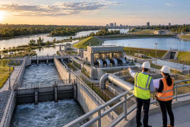
Software platforms such as HEC-RAS and Delft3D Flexible Mesh offer useful capabilities for these workflows.
HEC-RAS supports integrated one-dimensional and two-dimensional river modeling, while Delft3D FM provides flexible-grid hydrodynamic capabilities for river, estuarine, and coastal environments.
The Future of Computational Hydraulics
River modeling continues to benefit from better environmental datasets and more powerful computing infrastructure.
High-performance computing can make larger or more detailed numerical experiments more practical.
Automated mesh generation, remote sensing, and increasingly accessible cloud computing can also improve workflow efficiency.
Machine learning offers additional possibilities, including faster surrogate models for selected prediction tasks and improved processing of observational data.
Still, these developments don’t eliminate the need for physical reasoning.
A machine-learning prediction or a high-resolution CFD result must be evaluated against reliable measurements and the intended use of the model.
The most promising direction is therefore a combination of established hydraulic physics, modern computational tools, and continuous observational verification.
Advanced computational hydraulics is transforming how engineers understand and manage complicated river environments.
By combining physical equations, detailed terrain information, numerical modeling, and field observations, modern simulations can reveal hydraulic behavior that simplified calculations may overlook.
Whether the goal is flood risk assessment, bridge design, sediment management, or river restoration, choosing the appropriate modeling approach makes a significant difference.
The most successful projects prioritize reliable data, efficient mesh design, realistic boundary conditions, and rigorous validation rather than computational complexity alone.
As simulation technologies continue improving, engineers will have more opportunities to investigate river behavior and make informed infrastructure decisions.
Ready to improve your next river modeling project? Start by reviewing your existing hydraulic data, identifying the most important flow processes, and selecting simulation methods that match your engineering objectives.